How to win your football manager league through linear programming
A rule-based approach to determine your winning squad
Football manager leagues are a test of strategy and decision-making, but what if we could use algorithms to give us an edge? In this article, we will explore how linear programming (LP) can be used to create a league-winning squad. Of course, there is no winning guarantee but as the Nobel Prize winner Daniel Kahnemann likes to point out in his books Thinking, Fast and Slow and Noise, rule-based approaches commonly outperform human judgment. So let’s dive in and learn how to use LP while putting together the ultimate football squad. You can find the corresponding Python code here.
 Football manager leagues are a test of strategy and decision-making, but what if we could use algorithms to give us an edge?
There are many variations of football manager leagues out there but the common aim of most of them is building the best-performing squad in the upcoming season on a constrained budget. The primary goal is therefore to fill our squad with players that we expect to perform well without exceeding the available budget. Additionally, there are game-specific constraints like the strict positional commitment of players (e.g. goalkeeper) or the restriction of tactical formations (e.g. 4–4–2). But before diving into the specifics of the problem, let’s sketch our approach to select the ultimate football manager league squad.
First, we will review the rules (boundary conditions) of our football manager game of choice and explore the available data. We will then identify a way to predict the players’ performance in the upcoming season and create our LP model to find the optimal combination of players for the squad. Finally, we will refine the LP model to implement our strategies and discuss further ideas to improve the optimization routine. The sections will thus be:
- Exploring the boundary conditions and available data
- Predicting the players’ performance
- Creating the LP model
- Refining the LP model
- Further ideas
1. Exploring the boundary conditions and available data
The player statistics and rules here are based on a real football manager game, in which 22 Bundesliga players have to be selected on a budget of 42.5 million euros. The 22 players need to consist of three goalkeepers, six defenders, eight midfielders, and five attackers, distributed among one of these tactical starting formations ((goal)–defense–midfield–attack):
- (1)–3–5–2
- (1)–4–5–1
- (1)–4–4–2
- (1)–4–3–3
- (1)–3–4–3
- (1)–5–3–2
- (1)–5–4–1
The players are rated with a number of points after each matchday according to their actual performance and can be bought before the season for their in-game market value with the lowest possible price being 0.5 million euros. Each player’s performance is thus equivalent to the number of points gathered throughout the season. For the season 2022/2023 the available players’ statistics were as displayed in Table 1.
| first_name | last_name | dob | club | position | price |
|---|---|---|---|---|---|
| ronael | pierre-gabriel | 13/06/1998 | 1. fsv mainz 05 | defense | 1.2 |
| ruben | vargas | 05/08/1998 | fc augsburg | midfield | 1.6 |
| salih | �zcan | 11/01/1998 | borussia dortmund | midfield | 3.2 |
| sebastien | haller | 22/06/1994 | borussia dortmund | attack | 6 |
| solomon | bonnah | 19/08/2003 | rb leipzig | defense | 0.5 |
| steffen | tigges | 31/07/1998 | 1. fc k�ln | attack | 1.6 |
| stevan | jovetic | 02/11/1989 | hertha bsc | attack | 2.2 |
| timo | baumgartl | 04/03/1996 | 1. fc union berlin | defense | 2.2 |
| tobias | strobl | 12/05/1990 | fc augsburg | midfield | 1 |
| wahid | faghir | 29/07/2003 | vfb stuttgart | attack | 1 |
Table 1: Statistics of ten exemplary players of the season 2022/2023. The available data are the first name, last name, date of birth (dob), club, position, and price.
Based on this data, we could already select our 22 Bundesliga players fulfilling the constraints imposed by the football manager league rules. However, our goal is not just to randomly select 22 rule-compliant players, but 22 rule-compliant players who maximize the expected points gathered in the upcoming season. We thus have an optimization problem with the objective of finding a team to maximize the expected number of points. But how can we predict the number of points we expect players to collect throughout the upcoming season?
2. Predicting the players’ performance
A rather straightforward and intuitive approach to predicting future performance is to use the past performance of the players. Luckily, the players’ statistics for the seasons 2019/2020, 2020/2021, and 2021/2022 with the points each player collected throughout the season are available to us as shown in Table 2.
| first_name | last_name | dob | club | position | points | price |
|---|---|---|---|---|---|---|
| ricardo | pepi | 09/01/2003 | fc augsburg | attack | -4 | 1.8 |
| gideon | jung | 12/09/1994 | spvgg greuther f�rth | defense | 2 | 1.2 |
| philipp | tschauner | 03/11/1985 | rb leipzig | goal | 2 | 0.5 |
| romario | r�sch | 01/07/1999 | 1. fsv mainz 05 | midfield | 2 | 0.5 |
| fisnik | asllani | 08/08/2002 | tsg hoffenheim | attack | 4 | 0.5 |
| kevin-prince | boateng | 06/03/1987 | hertha bsc | midfield | 17 | 2.2 |
| dominik | kohr | 31/01/1994 | 1. fsv mainz 05 | midfield | 80 | 1.7 |
| taiwo | awoniyi | 12/08/1997 | 1. fc union berlin | attack | 198 | 2 |
| tjark | ernst | 15/03/2003 | vfl bochum | goal | nan | 0.5 |
| tom | weilandt | 27/04/1992 | vfl bochum | midfield | nan | 0.8 |
Table 2: Statistics of ten exemplary players of the season 2021/2022. As the season has passed already, each player has their accumulated number of points displayed. Players have “nan” points if they weren’t rated.
We can merge the tables of the seasons 2019/2020, 2020/2021, and 2021/2022 on the table of the current season 2022/2023 using the first name, last name, and date of birth as unique identifiers so that we end up with the table shown in Table 3 that contains the points each player collected in the previous seasons with the other stats being from the current season.
| first_name | last_name | dob | points_2019 | points_2020 | points_2021 | club | position | price |
|---|---|---|---|---|---|---|---|---|
| sardar | azmoun | 01/01/1995 | nan | nan | 37.0 | bayer 04 leverkusen | attack | 2.2 |
| mahmoud | dahoud | 01/01/1996 | 15.0 | 51.0 | 106.0 | borussia dortmund | midfield | 2.4 |
| benjamin | goller | 01/01/1999 | 6.0 | nan | nan | werder bremen | midfield | 0.8 |
| conor | noß | 01/01/2001 | nan | nan | 6.0 | bor. mönchengladbach | midfield | 0.6 |
| dong-jun | lee | 01/02/1997 | nan | nan | 0.0 | hertha bsc | attack | 0.7 |
| patrick | osterhage | 01/02/2000 | nan | nan | 32.0 | vfl bochum | midfield | 1.0 |
| maximilian | philipp | 01/03/1994 | nan | 69.0 | 38.0 | vfl wolfsburg | midfield | 2.0 |
| niklas | schmidt | 01/03/1998 | nan | nan | nan | werder bremen | midfield | 1.0 |
| sebastian | polter | 01/04/1991 | 8.0 | nan | 108.0 | fc schalke 04 | attack | 1.8 |
| philipp | pentke | 01/05/1985 | 31.0 | 18.0 | 6.0 | tsg hoffenheim | goal | 0.8 |
Table 3: Merged statistics of ten exemplary players of the past and upcoming seasons. As some players have not played all seasons (or none) they have “nan” points displayed.
To predict the future performance of a player we will take the points a player has gathered in past seasons and compute a weighted average that overweights the performance in more recent seasons. A reasonable choice to calculate the weights is to measure the correlation between the points players collected in one season with the points the players collected in the following seasons. More specifically we compute the correlation between the columns “points_2019” and “points_2020” (), “points_2020” and “points_2021” (), and “points_2019” and “points_2021” ():
We can now take the average of and as the average correlation between two consecutive seasons and as the correlation between seasons that are two years apart. Unfortunately, we cannot compute the correlation between seasons that are three years apart in the same way. However, we need to estimate the influence of the performance in the season 2019/2020 on the predicted performance in 2022/2023. Therefore, we will estimate it from the rate of change between and assuming an exponential decay of the correlation yielding
The weights required to calculate the weighted average are obtained by normalizing the sum of the correlations to 1:
Now, we have everything required to predict the number of points
collected in the upcoming season derived from the points of the past seasons (2019/2020), (2020/2021), and (2021/2022). We give players with missing points a default rating of 0 points so that each player has a performance prediction as it is shown in Table 4. We can now continue finding the squad that maximizes the number of predicted points given the constraints imposed by the football manager league rules.
| first_name | last_name | dob | points_2019 | points_2020 | points_2021 | club | position | price | prediction |
|---|---|---|---|---|---|---|---|---|---|
| sardar | azmoun | 01/01/1995 | 0.0 | 0.0 | 37.0 | bayer 04 leverkusen | attack | 2.2 | 17.664524722198465 |
| mahmoud | dahoud | 01/01/1996 | 15.0 | 51.0 | 106.0 | borussia dortmund | midfield | 2.4 | 69.78121459131805 |
| benjamin | goller | 01/01/1999 | 6.0 | 0.0 | 0.0 | werder bremen | midfield | 0.8 | 1.2461437830727382 |
| conor | noß | 01/01/2001 | 0.0 | 0.0 | 6.0 | bor. mönchengladbach | midfield | 0.6 | 2.86451752251867 |
| dong-jun | lee | 01/02/1997 | 0.0 | 0.0 | 0.0 | hertha bsc | attack | 0.7 | 0.0 |
| patrick | osterhage | 01/02/2000 | 0.0 | 0.0 | 32.0 | vfl bochum | midfield | 1.0 | 15.27742678676624 |
| maximilian | philipp | 01/03/1994 | 0.0 | 69.0 | 38.0 | vfl wolfsburg | midfield | 2.0 | 39.86933929498372 |
| niklas | schmidt | 01/03/1998 | 0.0 | 0.0 | 0.0 | werder bremen | midfield | 1.0 | 0.0 |
| sebastian | polter | 01/04/1991 | 8.0 | 0.0 | 108.0 | fc schalke 04 | attack | 1.8 | 53.22284044943304 |
| philipp | pentke | 01/05/1985 | 31.0 | 18.0 | 6.0 | tsg hoffenheim | goal | 0.8 | 14.97094315162026 |
Table 4: Merged statistics of ten exemplary players of the past and upcoming seasons. The column “prediction” contains the expected number of points for each player for the upcoming season.
3. Creating the LP model
In the season 2022/2023, there were players available for which we predicted the performance in the upcoming season. In order to find the squad that maximizes the number of expected points under the given constraints we have to formulate the problem in more mathematical terms.
We begin by defining a variable that is if a player is part of our optimal squad or if he is not. As we know, each of the players has a market value (price) and a predicted number of points . Furthermore, we know whether a player is a goalkeeper () or not (), a defender () or not (), a midfielder () or not (), or an attacker () or not (). This is already enough to formulate our objective function
that we want to optimize (maximize) and our constraints, which are
- do not exceed the budget:
- have three goalies:
- have six defenders:
- have eight midfielders:
- have five attackers:
The brute-force approach to this problem is trying every possible combination of 22 players and saving the one that maximized our objective function. However, choosing 22 from 553 players allows about possible combinations. So a brute-force approach is not even feasible with the most powerful computers. Luckily, LP, or more specifically binary LP (BLP), is here to help us out.
LP is a method for optimizing a linear objective function (here ), subject to constraints represented by linear equations or inequalities. The goal is to find the values of the variables (here ) that minimize or maximize the objective function, subject to the constraints. In our case, we speak of BLP since our variables can only take the binary values or (select a player or not), but more generally it is also possible to use LP if is an integer (integer LP or ILP) or continuous. We see that BLP is exactly what we need to efficiently solve our optimization problem and find our ideal squad.
In our case, we use the linear programming Python package PuLP to pick the players that will give us the number of predicted points while obeying the rules of the game. The implementation is rather simple with some knowledge of Python and the PuLP-specific syntax (see here).
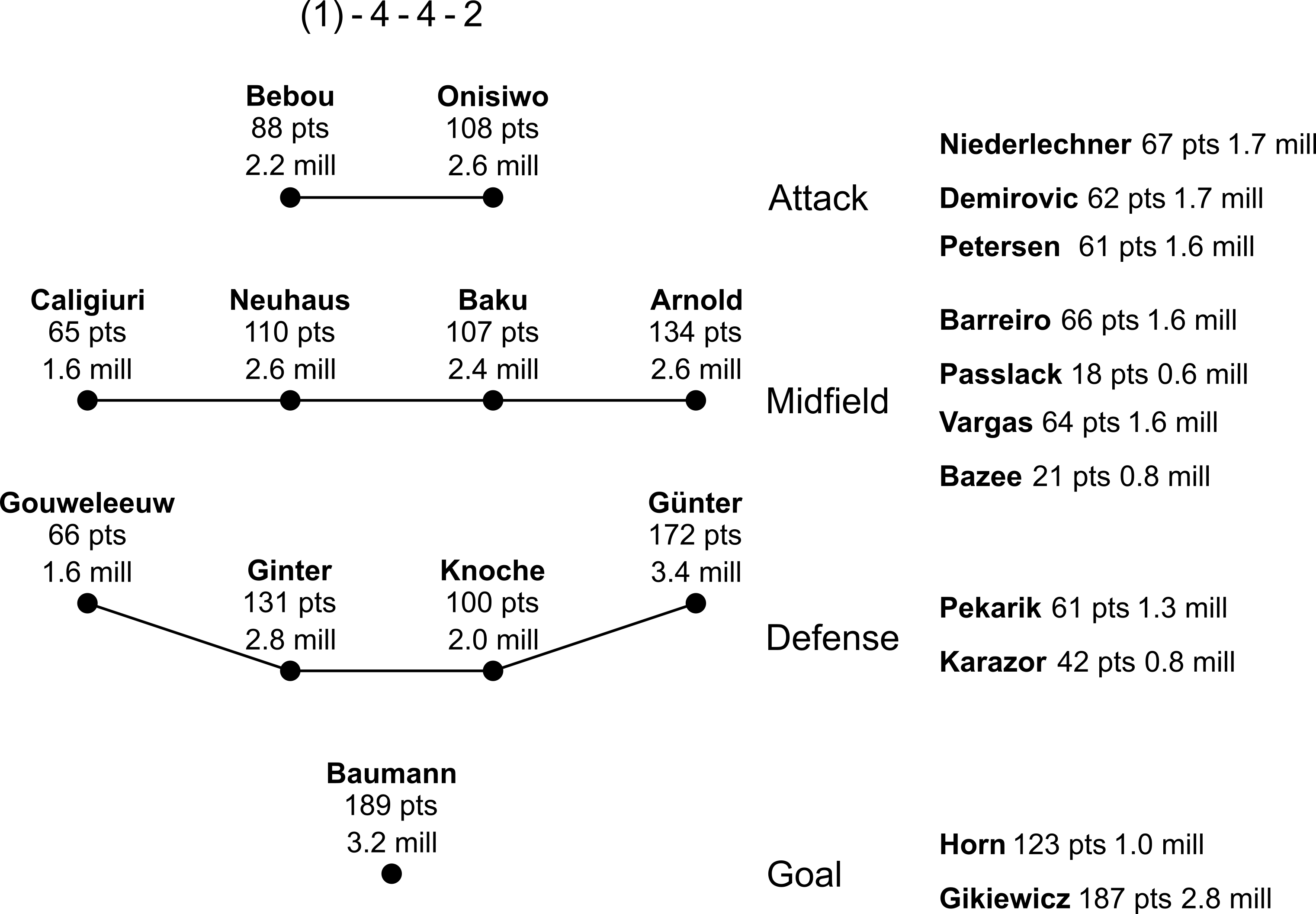 Figure 1: The team determined by our linear programming model that maximizes the number of predicted points. The tactical formation (1)–4–4–2 is exemplary here and could be replaced by any other formation.
Our LP model returns us the optimal 22 players shown in Figure 1 in practically no time. We can see that the squad is nicely balanced with decent players from various clubs and without pricy superstars. However, on each match day, only the points collected by the starting eleven are counted. This raises the question of whether we really need to have so many good substitutes. Wouldn’t it be better to spend more money on the starting eleven and save on some of the substitutes? It’s time to implement our personal strategies into the LP model.
4. Refining the LP model
The most straightforward approach to spending more money on the starters is to remove all substitutes. While the game requires us to buy 22 players we could just buy eleven substitutes for the minimal market value of 0.5 million euros and spend the remaining 42.5 - 11 ⋅ 0.5 = 37 million euros on the starters. The problem with that strategy is that players are often injured, have problems with a new coach, or are hindered to reach their old performance for other reasons. Because of that, it is smarter to at least have some decent substitutes.
A good compromise is to allow one drop-out of a player at each position. Intuitively, one could think that we thus need to buy four substitutes — one for each position. However, as we can change the tactical formation throughout the season it is actually enough to buy two substitute players — a goalkeeper and a field player. The list below shows the different tactical formations available with the corresponding positions of the two substitutes (subs) and the resulting tactical formation of core players (combined starters and subs)
- (1)–3–5–2 starters, (1)–1–0–0 subs → (2)–4–5–2 core players
- (1)–4–5–1 starters, (1)–0–0–1 subs → (2)–4–5–2 core players
- (1)–4–4–2 starters, (1)–0–1–0 subs → (2)–4–5–2 core players
- (1)–4–3–3 starters, (1)–0–1–0 subs → (2)–4–4–3 core players
- (1)–3–4–3 starters, (1)–1–0–0 subs → (2)–4–4–3 core players
- (1)–5–3–2 starters, (1)–0–1–0 subs → (2)–5–4–2 core players
- (1)–5–4–1 starters, (1)–0–0–1 subs → (2)–5–4–2 core players
We can see that the seven starter tactical formations can be reduced to three core tactical formations, which are (2)–4–5–2, (2)–4–4–3, and (2)–5–4–2. These core tactical formations ensure that eleven decent starters are available if up to one player in any position drops out. If we play with the starter tactical formation (1)–4–4–2 (core tactical formation (2)–4–5–2) and one of our attackers drops out, we can bring on our substitution midfielder and continue playing with a (1)–4–5–1 starter tactical formation. This works for any position and is great news as it gives us more flexibility and allows us to spend more money on our 13 core players.
The second strategic implementation is to ensure that we select players from different clubs. This is important for reasons of diversification. If we would select too many players from a single club the risk would be high to be strongly affected by a seasonal club crisis. One can argue (or validate from historical data) what a good upper limit of players from the same club is but here we use a quite low limit of two core players per club.
Let’s now refine our BLP model with our two strategic implementations: the reduction to thirteen core players and the limitation of two core players per club.
Our objective function to maximize stays as before
However, we need to update our constraints. For this, we need to introduce some new variables. Firstly, we define as the minimal market value in million euros. The binary parameter defines whether a player is playing on the -th position (goal , defense , midfield , attack ) or not with being the number of players on a position for each tactical formation. For the core tactical formation (2)–4–5–2 it is thus , , , and . We compute the number of cheap residual players as . Finally, we define as a binary parameter specifying whether a player plays in the club or not (the Bundesliga has 18 teams).
We have therefore three constraints for each of the three core tactical formations that refine our LP model to consider our personal strategy:
- do not exceed the budget:
- fulfill the position constraint:
- fulfill the club constraint:
Note, that the second constraint here is a more compact and flexible way to write the constraints 2–5 in the previous section. In Figure 2–4 you find the optimal squads determined by our refined LP model for the three core tactical formations. You can see that by sacrificing substitutes we could drastically increase the average number of core player points. All three formations have about the same number of total expected points so at this point the squad selection depends mostly on your personal taste.
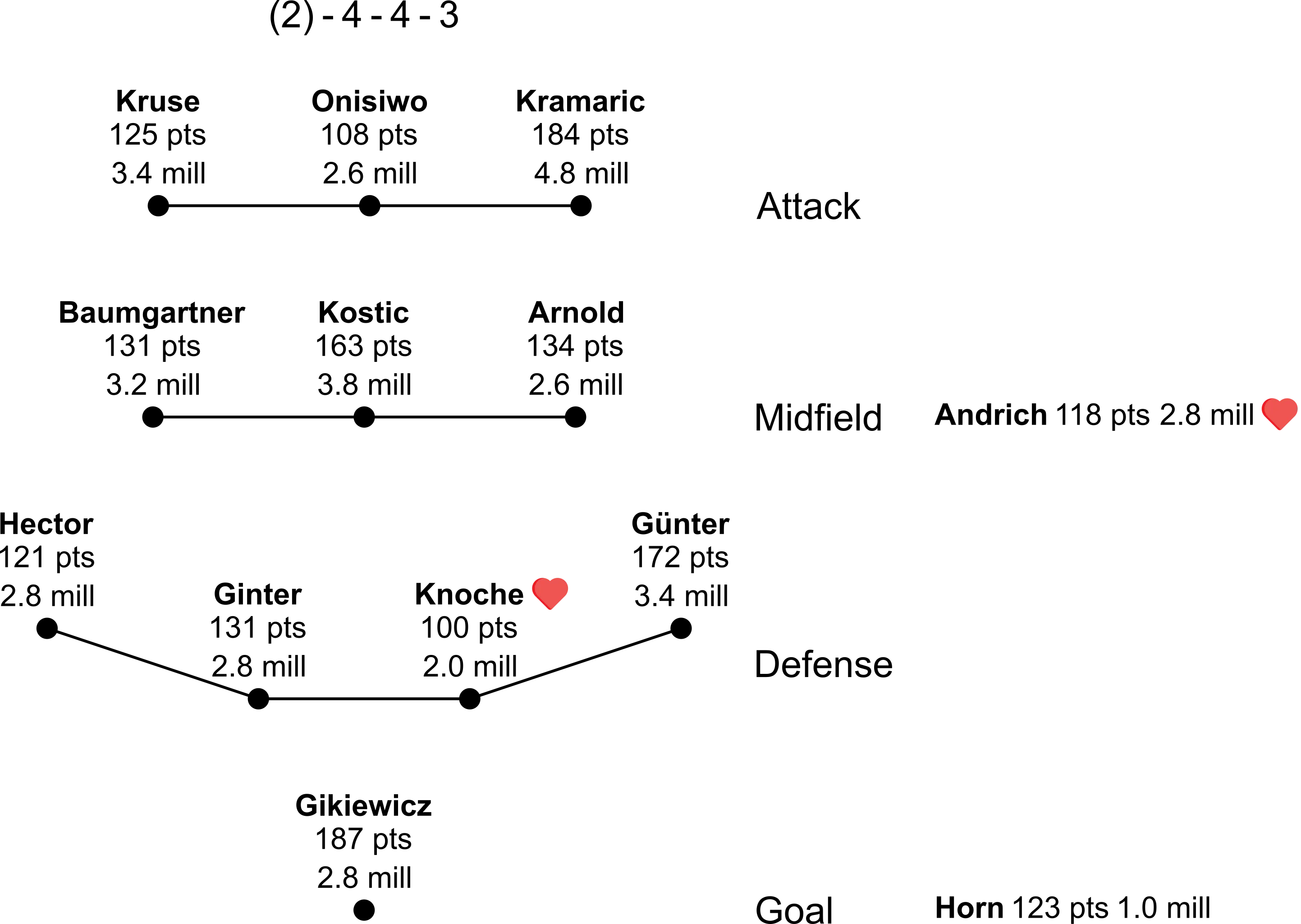 Figure 2: The team determined by our linear programming model that maximizes the number of predicted points for the core tactical formation (2)–4–4–3 considering our strategic implementations. The starter tactical formation (1)–4–3–3 is exemplary here and could be replaced by (1)–3–4–3 for example by substituting the players marked with a heart.
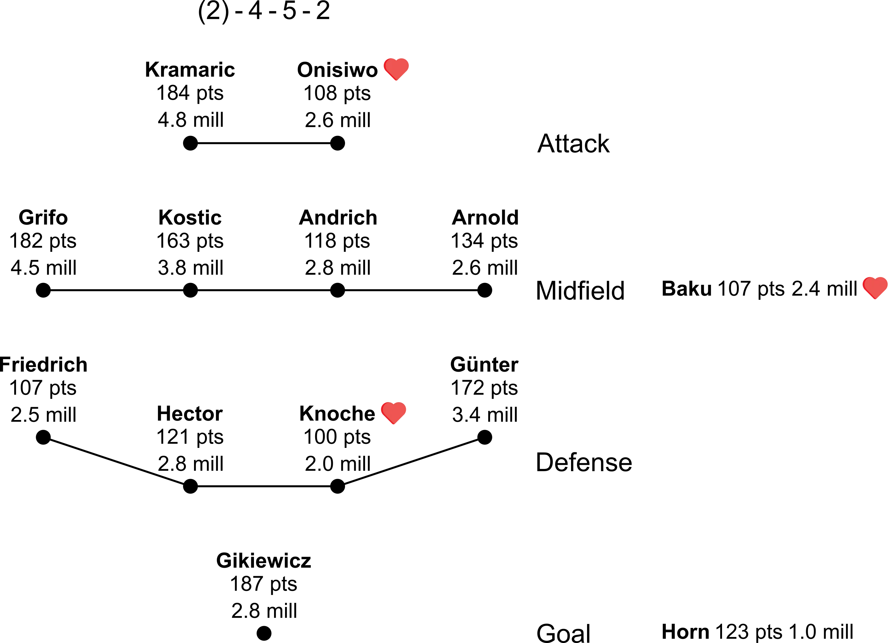 Figure 3: The team determined by our linear programming model that maximizes the number of predicted points for the core tactical formation (2)–4–5–2 considering our strategic implementations. The starter tactical formation (1)–4–4–2 is exemplary here and could be replaced by (1)–4–5–1 or (1)–3–5–2 for example by substituting the players marked with a heart.
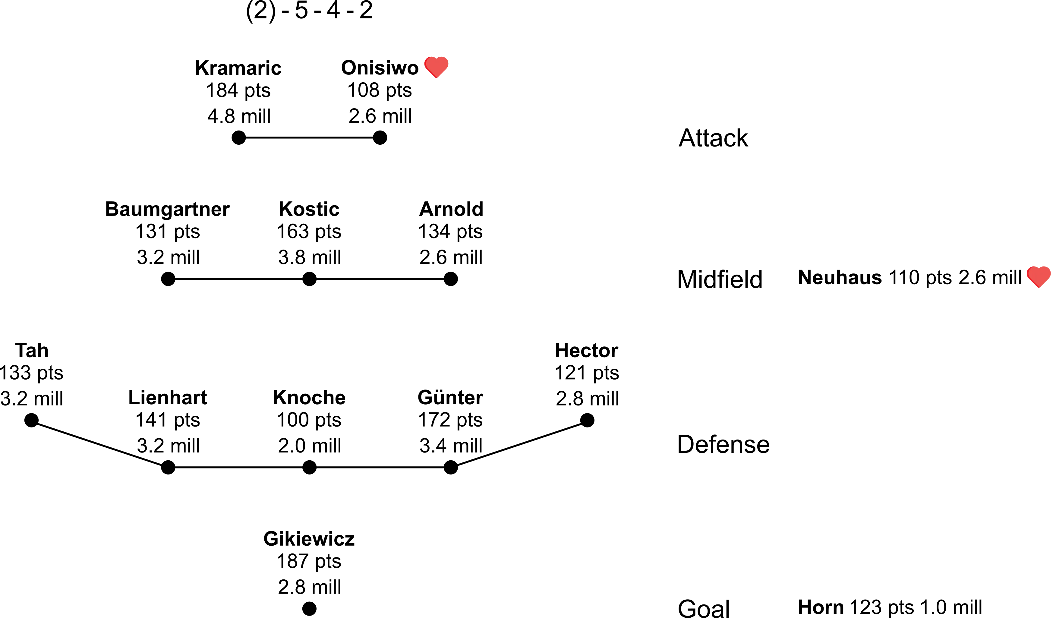 Figure 4: The team determined by our linear programming model that maximizes the number of predicted points for the core tactical formation (2)–5–4–2 considering our strategic implementations. The starter tactical formation (1)–5–3–2 is exemplary here and could be replaced by (1)–5–4–1 for example by substituting the players marked with a heart.
The refined BLP model already efficiently provides strong teams obeying the game rules and our personal strategy. Nevertheless, there is always room for improvement. So let’s discuss some ideas for future implementation before coming to an end.
5. Further ideas
A pretty simple but important update would be to allow blacklisting players from the whole optimization routine. This is because some players change to other leagues, have long-term injuries, or are not considered anymore. Goalkeeper Timo Horn is an excellent example of this, as he played well in previous seasons but was degraded to second goalkeeper this season. This explains his high number of predicted points but the low in-game market value in the squads above (Figure 1–4). Therefore, it makes sense to re-run the BLP optimization without these players.
Another quite interesting implementation would be to allow more than one player drop-out per position. In my experience, it is often not enough to allow only one missing player, requiring us to bring in a cheap residual player, and costing valuable points. Adding the capability to predict optimal squads for different numbers of player drop-outs would add a lot of flexibility to the squad. Similar to the limit of core players per club the ideal trade-off could be validated from historical data.
Being able to predict player performance from data that is not coming only from the Bundesliga would also be a major advantage. This is because the current approach does not allow for predicting the performance of players that were just transferred to the Bundesliga (see Sebastien Haller in Table 3) in a meaningful way. How difficult this is to implement depends on whether there is a database providing reliable match-wise player performance ratings. A football league rating could help normalize the player ratings to the league strength potentially providing good predictive power.
Do you have any other ideas on how to improve the BLP optimization pipeline? If so, let me know so that I can outcompete even my most talented (or lucky?) friends in the future :-) Also, don’t hesitate to reach out for corrections, additions, or questions. You can find the full Python code and data here.